590 Fall 2026 Week 8: 10/27-10/29/26. Changing the graph paper.

Agenda

• Yifan on PENTA and Dutch
• Common transformations for tone/intonation
• Intro to normalization and transforms
• Modeling normalization example: C-CURE
• Next week prep: watch neural nets videos; on horizon: lab on first half of class coming in next week

Transforms for fundamental frequency

Rose (1987): Considerations in the normalisation of fundamental frequency of linguistic tone

• Emphasis on normalization for vowels compared to tones/intonation still true today

  In contrast to the large amount of theoretical and empirical work done on vowel normalisation, the normalisation of the acoustical correlates of intonation has received very little attention, and the normalisation of tone even less. This is a pity, because without normalisation it is not possible to take the first step in defining the phonetic and phonological features of a particular variety, namely, separating those features of the acoustic signal which are characteristic of the individual from those which characterise the particular variety. (Rose, 1987, p. 344)

• What is the purpose of normalization?

  Vowel normalisation aims for a maximum reduction in B-S [between speaker] variance without sacrificing the desideratum of making perceptual sense. The notion of perceptual sense, which thus serves to evaluate the numerical strategy, can be understood in two ways: normalised values should correctly reflect the transcriber's auditory impression (Disner, 1980, p. 256), and normalisation should ideally model the actual process of the listener's perceptual normalisation. (Rose, 1987, p. 347)

  • However, Rose points out that it is hard to judge on the basis of perceptual criteria, because we still don't have a grasp of all the acoustic properties beyond f0 that contribute to pitch perception (that is still true! and a good point about how f0 is an abstraction)

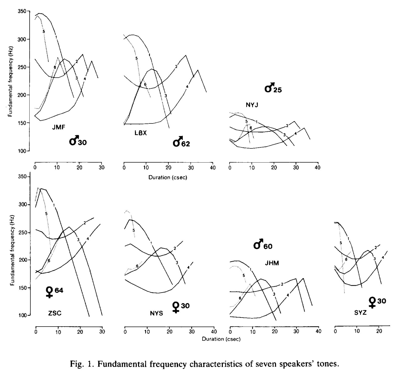
• Compare Rose (1987), Figure 1, mean raw f0 traces below of seven speakers of Zhenhai (Wu--see Rose's Wu tones page!) which has an inventory of 6 tones to z-scored f0 traces, tone f0 contour shapes taken from page 345:

  • T1: high falling
  • T2: level than rising in mid pitch range
  • T3: convex in low half o pitch range
  • T4: low rising into mid pitch range
  • T5: very high level or high falling
  • T6: short low rising into mid pith range
    

Normalization transformations

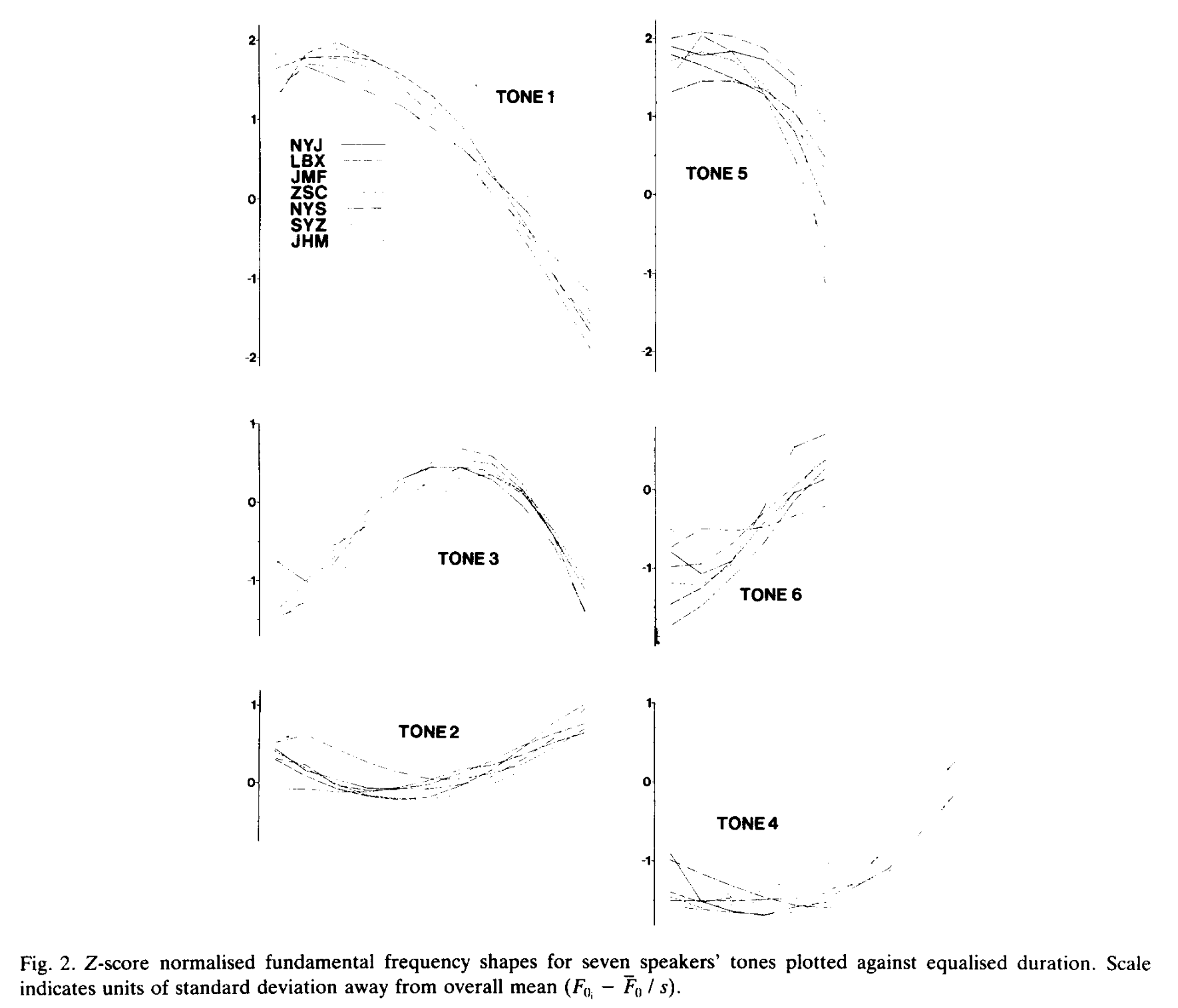
• What values should be considered for characterizing an individual speaker's f0 distribution? How do you "subtract" away the effect of an individual?
• Rose (1987) gives a general equation, which two more specific versions of transformations to consider: fraction of range (FOR) and z-scores.
• Here is the general equation:
  • \(\text{F0}_i\) refers to the \(i\)th F0 value in the F0 trajectory
  • \(\text{F0}_{ref}\) refers to some reference F0 value
  • \(\text{F0}_{range}\) refers to some operationalization of F0 range (or more generally, some estimate of the speaker's F0 distribution)

\[\text{F0}_{norm, i} = \frac{\text{F0}_i - \text{F0}_{ref}}{\text{F0}_{range}}\]

• Now here are the specific versions
• Fraction of range: \(\text{F0}_{range}\) is estimated using point estimates for maximum F0 and minimum F0

\[\text{F0}_{norm, i} = \frac{\text{F0}_i - \text{F0}_{min}}{\text{F0}_{max} - \text{F0}_{min}}\]

• z-scores: \(\text{F0}_{range}\) is estimated using the whole distribution, where \(\overline{\text{F0}}\) is the mean F0, and \(s\) is one standard deviation about the mean.

\[\text{F0}_{norm, i} = \frac{\text{F0}_i - \overline{\text{F0}}}{s}\]

• In what sense is standard deviation a way to operationalize range? Play with this Desmos normal distiribution notebook.
• Note that the mean and standard deviation are sufficient statistics for a Gaussian/normal distribution, see Table 3.1 below from Duda, Hart, and Stork (2001): they alone provide all the information about the sample for estimating the population.

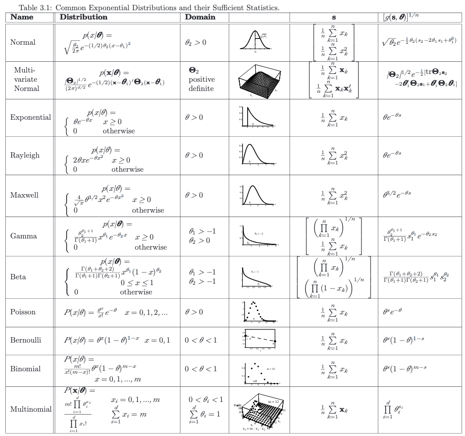
• The question for both of these normalization transforms is what values should be consiered in characterizing the f0 distribution?

• For FOR range values, Rose (1987, p. 348) points out:

  Range-defining (RD) points are values that are assumed to be equivalent between speakers, but unless they can be identified by external criteria, the normalisation becomes circular. (An FOR normalisation requires R-D points, but which points are equivalent between speakers only becomes clear after normalisation.)

  • Also extreme values could be outliers, e.g., from segmental perturbation or nonmodal phonation
  • Taking points that have low within-speaker variance? What happens if we take T1 offset as \(\text{F0}_{min}\) (which is a point of low within-speaker standard deviation)?

• For z-scores, Rose (1987) says:

  The NPs [normalization parameters] were calculated for each speaker from the set of his sampled mean F0 values in Table 1, excluding values at onset (0%), and offset (100%) in T5 (i.e., 49 data points for each speaker).” (Rose, 1987, p. 349)

  • And points out:

  ...as Disner (1980, p. 257) has pointed out for normalisations of different vowel systems, Z-score NPs should only be calculated from samples that are comparable (i.e., transcriptionally equivalent) to avoid biasing.” (Rose, 1987, p. 348)

  • But what counts as comparable?
  • Typically people just take all F0 values from a speaker to compute mean and standard deviation for z-scores: it's a bag of F0 values. What could be problems with that?

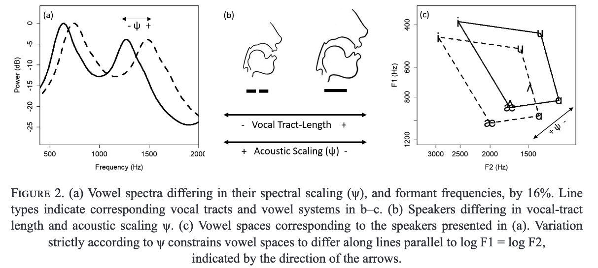
• FOR and z-score transformations are called affine transformations (linear transformations + translation), and are an example of "changing the graph paper".

• See also Wu (1999) p. 45, Section 3.2, Normalisation...

Changing the graph paper

The key idea: if we had the "right graph paper", then the relations between phonological categories would be "simpler"---we'd reveal systematic patterns that wouldn't otherwise be as apparent if we had a less-optimal graph paper for understanding how the categories lie in space. And maybe speakers/listeners use this graph paper too!

• What do we mean by changing the graph paper? Follow a vector!
  • Starting with 1D on the number line:
  • Transformations of the number line: see also text/video from Khan academy

• Functions as transformations: linear transformations video and page

  • Transformations in 2D: follow a point and see text/video from Khan academy
  • All you need to know is how transformations affect the basis vectors (or see Matrices section on linear transformations page!

• See physical graph paper

  • Polar coordinates and sinusoids
  • Cartesian to polar coordinates Desmos notebook
  • Polar to Cartesian coordinates Desmos notebook
  • Cardiod as a polar equation vs. on the Cartesian plane
  • various animations, especially the one below:

• Multiplicative between-speaker relationships: Barreda 2022 p. 2-4

  The uniform scaling hypothesis (also known as the constant ratio hypothesis) is one of the earliest attempts to explain phone-preserving variation in formant patterns, its general outlines being suggested at least as far back as Lloyd 1890. The uniform scaling hypothesis states that the perceived quality of vowel sounds is more likely to be maintained when variation in formant patterns is according to a single scaling parameter, relative to uncoordinated changes to individual formant frequencies.

  Variation of formant patterns according to a single spectral-scaling parameter (i.e. uniform scaling) results in spectra that differ in the expansion or contraction of a fixed pattern along the frequency axis, as in Figure 2a. Another way to look at this is that a single vowel quality can be associated with spectra differing in their ‘size’ expansion along the frequency axis, so long as their general, underlying spectral ‘shape’ is preserved (Irino & Patterson 2002).

  

  • \[F_{VS} = V_v \times \psi_s\] where \(V_v\) is the "underlying spectral shape" associated with some vowel quality \(v\) and \(F_{VS}\) is the "format pattern produced by speaker \(s\) for this vowel" and \(\psi_s\) is a "speaker-specific spectral-scaling parameter"

  Here, between-speaker variation in ψ is discussed directly in terms of proportional differences in expected formant frequencies, so if the ψs of one speaker is 10% higher than that of another, the first speaker is expected to produce formants that are 10% higher overall than those of the second speaker for any given vowel phoneme.

  The uniform scaling hypothesis does not imply that all between-speaker variation in formant patterns for a phoneme should be according to uniform scaling, but rather that these differences are most likely to preserve vowel quality.

Changing the graph paper: exercise from Mark Liberman COGS501

• See R notebook 590-F26-graph-paper-exploration.Rmd in code/w8_norm in Google Drive folder.
• Acoustic, "data-analytic" approach

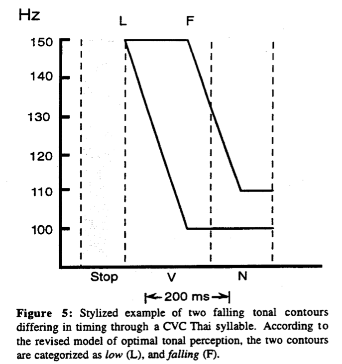
What's the clock? Does the clock vary?

• Absolute time, e.g., in ms, like a constant sampling rate over all utterances, not conditioned on any factors, no change over different domains
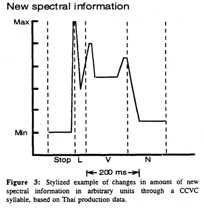
• "Phonological" time, e.g., segment out phonological units like the onset, rime, nucleus, segments, etc.
  • Then "normalize" over the phonological unit! (typically linear -> see Praat demo)
  • Constant sampling rate over each phonological unit across some population of utterances, e.g., across speakers, across tones, etc.
    
  • (Then what happens to absolute duration as a piece of information? You can add this information in separately in regressions...but is that sufficient for modeling what's happening?)

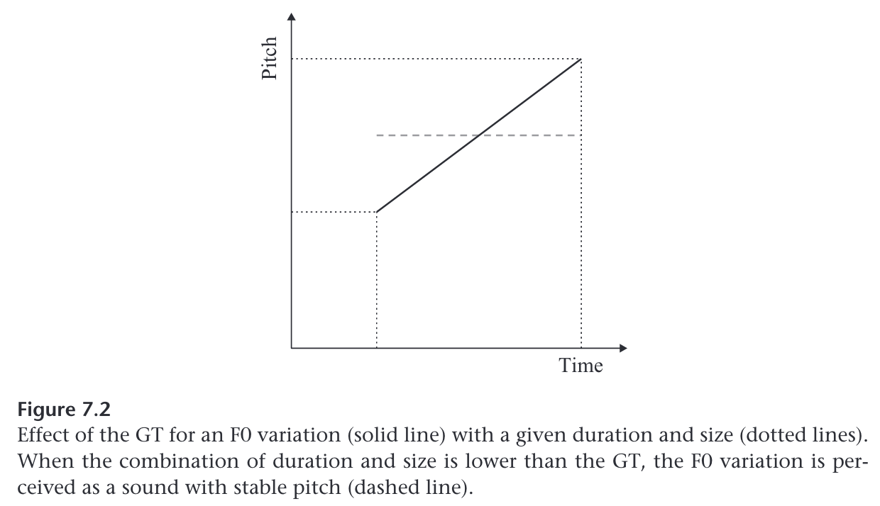
Perceptual motivation for clock choices

• See for instance some chapters in Prosodic Theory and Practice

• Schweitzer et al. (2022) on two different time normalization procedures for their "pitch stylization" algorithm

  PaIntE provides several methods to normalize the time axis. In the standard variant, which is called sylnorm normalization, the time axis inside the approximation window is normalized such that syllable boundaries occur at integer values, with the syllable related to the intonation event beginning at 0 and ending at 1. In the sylnorm case, b determines the temporal alignment of the peak in terms of relative position within the syllables in the approximation window. A hypothetical example peak contour for a syllable associated with a pitch accent, using sylnorm normalization, is given in figure 10.1. (p. 354-355)

  

  So far we have discussed only the application of PaIntE using the sylnorm normalization; however, PaIntE also provides an alternative called anchor normalization. In this case, each syllable is split into three parts representing the (unvoiced) onset of the syllable; its sonorant nucleus, which is defined as containing the nucleus and possibly preceding voiced consonants in the onset; and, finally, the coda. This normalization is motivated by findings that indicate that timing in F0 movements is relative to syllable structure (House 1996, 1997; van Santen and Möbius 2000). Using anchor normalization, each syllable in the approximation window is again normalized to length one with the same values for syllable boundaries as in the sylnorm case. Syllable-internally, the unvoiced onset is adjusted linearly to a length of 30 percent of the syllable duration. The sonorant nucleus then spans another 50 percent: it ranges from 30 to 80 percent of the syllable duration, and the coda finally goes from 80 to 100 percent of the syllable duration. (Schweitzer et al. 2022, p. 356-357)

  • Mertens p. 263 on spectral instability

  Spectral instability and its impact on pitch perception. Spectral change and amplitude drop at the transition between sounds (consonants and vowels) can perceptually mask F0 change during this transition (’t Hart, Collier, and Cohen 1990, 36). Experiments by House (1990) show that an F0 variation—for instance, a linear rise of fixed duration and size—is perceived differently, as either a pitch movement or an abrupt change of pitch, depending on its location relative to the vowel onset in the syllable. This phenomenon (known as the spectral stability hypothesis) is attributed to spectral change at the transition between sounds, which lowers sensitivity to pitch change. The amount of spectral change at sound transitions depends on the nature of the sounds involved; nasals and liquids are more similar to vowels than fricatives, for instance. A more detailed segmentation model based on spectral change also takes into account the nature of the sounds in the syllable rhyme (House 1995, 1996). This perceptual phenomenon explains why hearers are able to distinguish pitch movements occurring between adjacent syllables from those occurring within one and the same syllable.

  

  

  • Mertens p. 263-264 on glissando

  Intrasyllabic pitch movement and the glissando threshold. Some syllables are perceived with a stable pitch, others with a changing pitch. In music, the latter type would be called a glissando. For a gliding pitch, the observed F0 change will exceed a threshold, which depends on the pitch interval covered by the glide and its duration (’t Hart, Collier, and Cohen 1990). Listening experiments with natural or synthetic speech (Rossi, 1971; Rossi et al. 1981; Mertens, Beaugendre, and d’Alessandro 1997) show that many intrasyllabic F0 variations observed in speech are indeed perceived. as glissandi. To decide whether a syllable is perceived with a stable or a gliding pitch, the combination of duration and size of the corresponding F0 variation is compared to the glissando threshold (GT), as illustrated for a uniform F0 change in figure 7.2. When they exceed the GT, a gliding pitch is obtained (solid line), otherwise a stable pitch is perceived with a frequency approaching the median F0 of the variation (dashed line).

  The GT was first observed and measured in experimental settings, using stimuli with known properties, such as pure tones or synthetic vowels, presented repeatedly, separated by silence, hence followed by a pause. Natural, continuous speech is characterized instead by spectral instability due to sound concatenation and by the occasional presence of pauses. As a result, the threshold is higher in connected speech than for isolated sounds. House (1995) shows that the presence of the pause facilitates pitch perception—in other words, it lowers the GT. (For a detailed description of the measurement of the GT, see d’Alessandro and Mertens 1995, section 2.5.2.)

Modeling normalization

• McMurray and Jongman (2011) compare/contrast three approaches:

  • "Naive invariance" model: small number of invariant acoustic properties, i.e., invariant with respect to context.

  • See for instance Sussman et al. 1998 on locus equations and commentary

    • Operationalized as follows, using linear regression with each acoustic properties as as dependent variable:

    “We next asked if any cues appeared more invariant than others. That is, are there cues that are correlated with a single feature (place of articulation, sibilance, or voicing) but not with context? There is no standard for what statistically constitutes an invariant cue, so we adopted a simple criterion based on Cohen and Cohen’s (1983) definition of effect sizes as small (R2 .05), medium (.05 R2 .15), and large (R2 .15): A cue is invariant if it had a large effect of a single feature (sibilance, place of articulation, voicing) and at most, small effects of context.” (McMurray and Jongman, 2011, p. 226)

  • Exemplar models: no difference in encoding of exemplar for acoustic properties that might index speaker identiy from ones that might cue phonological contrast, also not clear how acoustic properties outside the window/domain are taken into account, e.g., information from neighboring segments/speech material

  • "Parsing" models, including C-CuRE

    The C-CuRE approach derives from a class of perceptual processes loosely identified as parsing. Parsing was first hinted at by Ohala (1981) and later developed by Fowler (1984; Fowler & Smith 1986) to deal with overlapping sources of variance in the speech signal, such as overlapping articulatory gestures. The idea is simple: at any given point in the signal, listeners assign acoustic cues to causes. Fowler’s version of parsing assumes these causes to be gestural; however, later instantiations of parsing (Gow 2003) take a less specific stance, arguing simply that similar acoustic cues (e.g. lowered F1) in different positions (e.g. syllable-finally, and at the onset of the next syllable) are grouped via association with features like labiality or coronality. Whether parsing is in terms of gestures or feature-cues, the “causes” can originate in the past or future (i.e. can precede or follow the target sound), or can be cotemporaneous with the target, with the result that parsing can have very powerful results for speech perception.” (McMurray, Cole, and Munson, 2011, p. 204)

Computing Cues Relative to Expectations, C-CuRE

• Idea: not all cues should be treated the same (or treated the same by listeners)! Some should be considered in context--doing so then reduces variation in the acoustic signal
• Implementation: "subtract out" effect of context for a given cue.
• Example, adapted from McMurray, Cole, and Munson (2011) p. 207-208: let's say we are looking at f0 as acoustic property, a cue for recognizing tone class. Let's assume two tone classes, High and Low. A linear regression with F0 as the dependent variable (let's say, just for illustrative purposes, F0 at the midpoint of the rime) would look like this:

\[ \text{F0}_{rime} = \beta_{0} + \beta_1 \cdot \text{tone} \]

where

• tone is the dummy-coded tone class variable, say, 1 for High and 0 for Low
• \(\beta_0\) is the y-intercept

• \(\beta_1\) is the slope

• From now on we're just going to write F0 for F0\(_{rime}\) to make the subscripts simpler.

• There are also other factors that affect F0, such as speaker identity, and the vowel (intrinsic F0 effects) and we include these as well in the linear regression:

\[ \text{F0} = \beta_{0,all} + \beta_{tone} \cdot \text{tone} + \beta_{speaker} \cdot \text{speaker} + \beta_{vowel} \cdot \text{vowel} \ldots \]

• Once we compute the linear regression we then get the \(\beta\) coefficient weights for each factor.
• Then we can use the equation to predict what value of F0 we expect, given the factors, i.e., given the tone class, the speaker, the vowel, etc. This gives us the expected value for F0, given the context/tone class
• We can then remove the effects of a source of variation in F0, say the speaker effect:

\[ \text{F0} = \beta_{0,speaker} + \beta_{1,speaker} \cdot \text{speaker} \]

Once we have computed the coefficients from the speaker-only linear regression, we can residualize F0:

\[ \text{F0}_{resid} = \text{F0}_{measured} - \left(\beta_{0,speaker} + \beta_{1,speaker} \cdot \text{speaker}\right) \]

• Then use the \(\text{F0}_{resid}\) as the new dependent variable in linear regression with other factors to see if the affect remaining variance in F0 after speaker effect is partialed out
• And use \(\text{F0}_{resid}\) as an independent variable in a linear regression taking residualized values as input for identifying tone classes.